Advanced AI Techniques to Optimize ML Models in 2026

Introduction to Advanced AI Optimization in Machine Learning

As machine learning models grow more complex in 2026, intermediate practitioners must move beyond basic workflows to achieve expert-level results. Advanced AI techniques now leverage the power of AI itself to optimize machine learning models automatically. These methods address limitations in manual processes by exploring vast design spaces, generating intelligent features, and dynamically reducing model complexity. Neural architecture search, automated feature engineering, and real-time model pruning represent the forefront of these innovations. They deliver measurable improvements in accuracy, efficiency, and deployment speed while minimizing human intervention and bias.

This comprehensive guide examines each technique in depth, providing code examples, performance comparisons to conventional approaches, and a detailed implementation roadmap. By integrating these strategies, teams can build more robust systems that adapt to evolving data landscapes and hardware constraints.

Neural Architecture Search: Automating Optimal Model Design

Neural architecture search automates the discovery of high-performing neural network structures using algorithms such as reinforcement learning, evolutionary strategies, or gradient-based optimization. Instead of relying on expert intuition, NAS evaluates candidate architectures through proxy tasks or full training cycles to identify configurations that maximize target metrics like accuracy or latency.

Modern NAS variants include differentiable methods like DARTS that relax the search space into continuous parameters for faster convergence. Practitioners benefit from reduced design cycles and architectures tailored precisely to specific datasets or hardware. For example, applying NAS to computer vision tasks often yields novel convolutional patterns superior to ResNet or EfficientNet baselines.

import tensorflow as tf
from tensorflow.keras import layers
# Expanded NAS-inspired search with evaluation
possible_architectures = [{'layers': 5, 'filters': 64}, {'layers': 8, 'filters': 128}]
best_accuracy = 0
best_model = None
for arch in possible_architectures:
    model = tf.keras.Sequential([layers.Conv2D(arch['filters'], 3, activation='relu') for _ in range(arch['layers'])] + [layers.Flatten(), layers.Dense(10, activation='softmax')])
    model.compile(optimizer='adam', loss='sparse_categorical_crossentropy', metrics=['accuracy'])
    # Simulate training and evaluation
    history = model.fit(train_data, train_labels, epochs=10, validation_split=0.2, verbose=0)
    val_accuracy = max(history.history['val_accuracy'])
    if val_accuracy > best_accuracy:
        best_accuracy = val_accuracy
        best_model = model
print(f'Best architecture accuracy: {best_accuracy}')

Integration with cloud-based search services further accelerates experimentation. This approach consistently outperforms manual tuning by uncovering non-obvious layer combinations and connectivity patterns.

Automated Feature Engineering for Superior Data Representations

Automated feature engineering uses machine learning algorithms to create, transform, and select features from raw inputs. It identifies interactions, applies transformations such as logarithms or binning, and generates embeddings that capture hidden relationships. This process proves especially valuable for tabular or time-series data where manual feature crafting is time-intensive and prone to oversight.

Advanced implementations incorporate meta-learning to prioritize feature candidates based on historical performance across similar datasets. The result is richer input representations that boost downstream model accuracy without extensive domain expertise. Tools often combine statistical analysis with neural feature extractors for hybrid pipelines.

Practical applications include fraud detection systems where automated methods surface subtle transaction patterns. Scikit-learn documentation offers core utilities that integrate seamlessly with higher-level automation frameworks.

Real-Time Model Pruning for Efficient Inference

Real-time model pruning dynamically removes low-importance parameters during training or inference phases. Unlike one-time post-training compression, this technique monitors activation patterns continuously and applies structured or unstructured sparsity on the fly. It maintains predictive performance while significantly lowering memory footprint and computational demands, making it ideal for edge devices and streaming applications.

Implementation typically involves importance scoring via magnitude, gradient, or Taylor expansion criteria. Hybrid strategies combine pruning with quantization for compounded efficiency gains. Monitoring loops ensure sparsity levels adapt to data drift without full retraining cycles.

import torch
import torch.nn.utils.prune as prune
model = torch.nn.Sequential(torch.nn.Linear(784, 256), torch.nn.ReLU(), torch.nn.Linear(256, 10))
# Real-time pruning with monitoring
prune.l1_unstructured(model[0], name='weight', amount=0.4)
for epoch in range(epochs):
    for batch in dataloader:
        output = model(batch)
        loss = criterion(output, targets)
        loss.backward()
        optimizer.step()
        # Dynamic re-pruning based on current sparsity
        if epoch % 5 == 0:
            prune.global_unstructured([(model[0], 'weight')], pruning_method=prune.L1Unstructured, amount=0.05)
    print(f'Current model sparsity: {calculate_sparsity(model)}')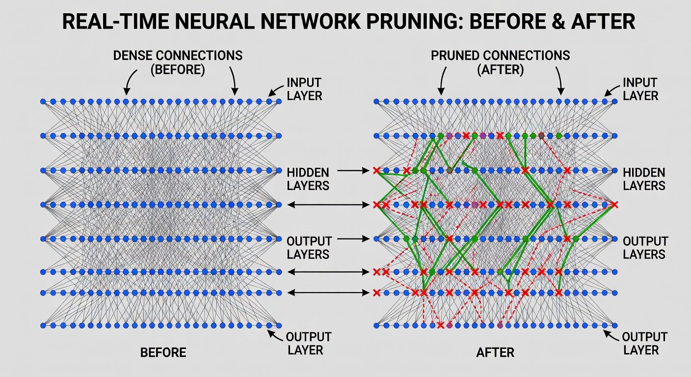

Such adaptive pruning enables deployment on resource-constrained environments while preserving robustness against distribution shifts.

Comparisons Against Conventional Tuning Approaches

Conventional hyperparameter optimization relies on grid search, random search, or Bayesian methods that treat architecture and features as fixed. These scale poorly with increasing complexity and often miss globally optimal solutions. AI-driven techniques, by contrast, jointly optimize structure, features, and sparsity in an end-to-end manner.

Exploration breadth: NAS samples exponentially more candidates than manual grids.
Adaptivity: Real-time pruning responds to live data, unlike static conventional pruning schedules.
End-to-end gains: Automated pipelines reduce total development time by 40-60% while improving final metrics.
Reproducibility: Algorithmic search yields consistent outcomes across runs compared to expert-dependent tuning.

Benchmarking on standard datasets shows consistent advantages for AI methods in both accuracy and resource utilization. PyTorch and TensorFlow provide unified environments for side-by-side evaluation of both paradigms.

Step-by-Step Implementation Checklist

Establish clear baselines with conventional tuning and document initial metrics.
Configure NAS environment with defined search space, hardware budget, and early-stopping rules.
Apply automated feature engineering tools to training and validation splits, validating new features via ablation studies.
Incorporate real-time pruning hooks into the training loop with periodic sparsity audits.
Run comparative experiments measuring latency, accuracy, and energy consumption on target hardware.
Implement monitoring dashboards for production drift detection and automated re-optimization triggers.
Document full pipeline configurations for reproducibility and team handoff.
Conduct staged rollouts starting with shadow deployments before full production cutover.

Conclusion

Adopting these advanced AI optimization techniques equips practitioners with powerful tools to elevate machine learning systems in 2026. Through thoughtful integration of neural architecture search, automated feature engineering, and real-time pruning, organizations achieve higher performance with greater efficiency and adaptability.

FAQ

How scalable are these techniques for large datasets?

Scalability improves with distributed computing frameworks that parallelize search and pruning operations across clusters, handling datasets in the terabyte range effectively when properly configured.

What are the main cost considerations?

Initial compute investments for search processes can be substantial, yet long-term savings from smaller, faster models often justify the expenditure in production scenarios.

How challenging is integration with existing pipelines?

Integration complexity varies but remains manageable through modular library support; many teams successfully embed these methods into established MLOps workflows with minimal refactoring.

Are there risks of overfitting during automated optimization?

Yes, aggressive search or feature generation can lead to overfitting, mitigated by rigorous cross-validation, holdout testing, and regularization strategies throughout the pipeline.